1. Prepare • extremeR

Introduction

Estimating the the models described in Explaining Recruitment to Violent Extremism: A Bayesian Case-Control Approach (ERVE) requires just two steps:

Prepare the data sources in list format using data.prep()
Estimate the model using fit()

This explainer vignette walks you through the first of these two steps.

Preparing the dataset for the estimation procedure requires two sources of data: 1) survey data with labels for “cases” and “controls” (as well as any relevant covariates) and; a shapefile for the geographical region under investigation.

Setup

First install the package from source if not already installed.

devtools::install_github("extremerpkg/extremeR")

We then load the package into memory as follows.

library(extremeR)

We can then load the data we need into memory using the data bundled in this package as follows.

data(survey_egypt)
data(shape_egypt)
data(denom_mena)

We can see that our case-control survey data, survey_egypt, and our denominator data, denom_mena are “data.table” “data.frame” objects.

Our Egypt shapefile data is here stored as an “sf” “data.frame” object.

class(survey_egypt)

## [1] "data.table" "data.frame"

class(shape_egypt)

## [1] "sf"         "data.frame"

class(denom_mena)

## [1] "data.table" "data.frame"

Note that here we are using data bundled with the extremeR package. If we had a series of shapefiles of the type provided e.g. here, we could generate the “sf” object from these files as follows.

shapefile_path <- "data/EGY_adm2.shp"
shape_egypt <- sf::st_read(shapefile_path)

Inspect data

Now that we have each data source that we need: i.e., the case-control data and the shapefile, we are ready to inspect the data. We will begin with the case-control data.

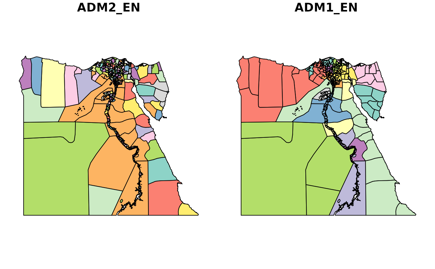
Here we see that our observations are labelled as either “0” if a control or “1” if a case. Alongside this information we have a series of relevant covariates. The last column in our data is the geographical region from which the observation is derived. We will use this last column to merge the data with the shapefile information.

The shapefile data is plotted below. The relevant geographic identifiers we’ll be using in the shapefile are “ADM1_EN” for the large area and “ADM2_EN” for the small area.

We’ll then be merging with the “ADM2_PCODE” identifier, as this is the common identifier between our shapefile and case-control data.

Finally, we need to input information on the known prevalence of the outcome in the population of interest. For this, we need to know the relevant population denominator. In the ERVE example, this is the adult male Sunni population.

These data are also bundled into the package, and we can look at them below.

To extract the relevant denominator for Egypt we can do as follows.

denom_egypt <- denom_mena$male_18_sunni[which(denom_mena$country=="Egypt")]

Preparing the data

We are now in a position to bundle these data sources into a list object suitable for the fit() function to estimate one of the models described in ERVE.

The data.prep() function has a series of parameters that we tabulate and describe below.

Argument	Description
shape	sf object, shapefile data
survey	data.table data.frame, case-control data including common geographic ID
shape_large.area_id_name	string, large area name identifiers in the shapefile
shape_large.area_id_num	integer, large area identifiers in the shapefile
shape_small.area_id_name	string, small area name identifiers in the shapefile
shape_small.area_id_num	integer, small area identifiers in the shapefile
survey_small.area_id_name	string, small area name identifiers in the survey
survey_small.area_id_num	integer, small area identifiers in the survey
drop.incomplete.records	logical, should the function return complete data? Defaults to `TRUE`
colnames_X	character vector, covariates definining the design matrix X. Must be numeric.
interactions_list	list, each element is a string of the form “a*b” where a and be are the names of two variables in colnames_X
scale_X	string, takes values “1sd” or “2sd”
colname_y	string, variable name for the outcome variable. Must be numeric.
contamination	logical, should this offset account for contamination? Defaults to `TRUE`
pi	numeric, scalar defining the prevalence of the outcome in the population of interest
large_area_shape	logical, should the function return a large-area shapefile? Defaults to `TRUE`

# prep data
data.list =
  data.prep(
    shape = shape_egypt,
    survey = survey_egypt,
    shape_large.area_id_name = "ADM1_EN",
    shape_large.area_id_num = NA,
    shape_small.area_id_name = "ADM2_EN",
    shape_small.area_id_num = "ADM2_PCODE",
    survey_small.area_id_name = NA,
    survey_small.area_id_num = "adm2_pcode",
    drop.incomplete.records = T,
    colnames_X = c(
      "coledu",
      "age",
      "married",
      "student",
      "lowstat",
      "population_density",
      "total_population_2006",
      "christian_2006_pct",
      "university_2006_pct",
      "agriculture_2006_pct",
      "mursi_vote_2012_pct",
      "sqrt_killed_at_rabaa",
      "unemployment_2013q4_pct",
      "sqrt_protest_post_Mubarak"
    ),
    interactions_list = list(age2 = "age*age", coledu_lowstat = "coledu*lowstat"),
    scale_X = "1sd",
    colname_y = "case",
    contamination = T,
    pi = 1000 / denom_egypt,
    large_area_shape = T
  )

The data.prep() function takes our shapefile and case-control data and bundles it into a list.

We can look at the structure of these data below. We see that the list contains our survey data, shapefiles, generated neighbourhood matrices, outcome observations etc.

summary(data.list)

##                    Length Class      Mode     
## survey_complete        20 data.table list     
## n                       1 -none-     numeric  
## y                     617 -none-     numeric  
## pi                      1 -none-     numeric  
## n1                      1 -none-     numeric  
## n0                      1 -none-     numeric  
## offset                  1 -none-     numeric  
## theta_1                 1 -none-     numeric  
## theta_0                 1 -none-     numeric  
## X                      17 data.table list     
## p                       1 -none-     numeric  
## mu_X                   16 -none-     numeric  
## sd_X                   16 -none-     numeric  
## scale_X                 1 -none-     character
## small_area_id         617 -none-     numeric  
## small_area_names      365 -none-     character
## large_area_id         617 -none-     numeric  
## large_area_names       27 -none-     character
## N_large_area            1 -none-     numeric  
## nb_object             365 nb         list     
## N_small_area            1 -none-     numeric  
## node1_small_area      824 -none-     numeric  
## node2_small_area      824 -none-     numeric  
## N_small_area_edges      1 -none-     numeric  
## scaling_factor          1 -none-     numeric  
## nb.matrix          133225 -none-     numeric  
## shape_small            20 sf         list     
## shape_large             2 sf         list

And we can save the formatted data for later use as follows.

save(data.list, "data/data.list.rda")

We can then check that the neighbourhood matrix is properly connected using the testconnected() function as below.

# check that the nb object is fully connected
testconnected(data.list$nb_object)

## [1] "Success! The Graph is Fully Connected"